Discrete called a random variable that can take on individual, isolated values with certain probabilities.
EXAMPLE 1. The number of times the coat of arms appears in three coin tosses. Possible values: 0, 1, 2, 3, their probabilities are equal respectively:
P(0) = ; Р(1) = ; Р(2) = ; Р(3) = .
EXAMPLE 2. The number of failed elements in a device consisting of five elements. Possible values: 0, 1, 2, 3, 4, 5; their probabilities depend on the reliability of each element.
Discrete random variable X can be given by a distribution series or a distribution function (the integral distribution law).
Near distribution is the set of all possible values Xi and their corresponding probabilities Ri = P(X = xi), it can be specified as a table:
| x i | x n |
|||
| p i | р n |
At the same time, the probabilities Ri satisfy the condition
Ri= 1 because 
where is the number of possible values n may be finite or infinite.
Graphical representation of the distribution series called the distribution polygon . To construct it, possible values of the random variable ( Xi) are plotted along the x-axis, and the probabilities Ri- along the ordinate axis; points Ai with coordinates ( Xi,рi) are connected by broken lines.
Distribution function random variable X called function F(X), whose value at the point X is equal to the probability that the random variable X will be less than this value X, that is
F(x) = P(X< х).
Function F(X) For discrete random variable calculated by the formula
F(X) = Ri , (1.10.1)
where the summation is carried out over all values i, for which Xi< х.
EXAMPLE 3. From a batch containing 100 products, of which there are 10 defective, five products are randomly selected to check their quality. Construct a series of distributions of a random number X defective products contained in the sample.
Solution. Since in the sample the number of defective products can be any integer ranging from 0 to 5 inclusive, then the possible values Xi random variable X are equal:
x 1 = 0, x 2 = 1, x 3 = 2, x 4 = 3, x 5 = 4, x 6 = 5.
Probability R(X = k) that the sample contains exactly k(k = 0, 1, 2, 3, 4, 5) defective products, equals
P (X = k) = .
As a result of calculations using this formula with an accuracy of 0.001, we obtain:
R 1 = P(X = 0) @ 0,583;R 2 = P(X = 1) @ 0,340;R 3 = P(X = 2) @ 0,070;
R 4 = P(X = 3) @ 0,007;R 5 = P(X= 4) @ 0;R 6 = P(X = 5) @ 0.
Using equality to check Rk=1, we make sure that the calculations and rounding were done correctly (see table).
| x i | ||||||
| p i |
EXAMPLE 4. Given a distribution series of a random variable X :
| x i | |||||
| p i |
Find the probability distribution function F(X) of this random variable and construct it.
Solution. If X£10 then F(X)= P(X<X) = 0;
if 10<X£20 then F(X)= P(X<X) = 0,2 ;
if 20<X£30 then F(X)= P(X<X) = 0,2 + 0,3 = 0,5 ;
if 30<X£40 then F(X)= P(X<X) = 0,2 + 0,3 + 0,35 = 0,85 ;
if 40<X£50 then F(X)= P(X<X) = 0,2 + 0,3 + 0,35 + 0,1=0,95 ;
If X> 50, then F(X)= P(X<X) = 0,2 + 0,3 + 0,35 + 0,1 + 0,05 = 1.
LAW OF DISTRIBUTION AND CHARACTERISTICS
RANDOM VARIABLES
Random variables, their classification and methods of description.
A random quantity is a quantity that, as a result of experiment, can take on one or another value, but which one is not known in advance. For a random variable, therefore, you can only specify values, one of which it will definitely take as a result of experiment. In what follows we will call these values possible values of the random variable. Since a random variable quantitatively characterizes the random result of an experiment, it can be considered as a quantitative characteristic of a random event.
Random variables are usually denoted by capital letters of the Latin alphabet, for example, X..Y..Z, and their possible values by corresponding small letters.
There are three types of random variables:
Discrete; Continuous; Mixed.
Discrete is a random variable whose number of possible values forms a countable set. In turn, a set whose elements can be numbered is called countable. The word "discrete" comes from the Latin discretus, meaning "discontinuous, consisting of separate parts".
Example 1. A discrete random variable is the number of defective parts X in a batch of nproducts. Indeed, the possible values of this random variable are a series of integers from 0 to n.
Example 2. A discrete random variable is the number of shots before the first hit on the target. Here, as in Example 1, the possible values can be numbered, although in the limiting case the possible value is an infinitely large number.
Continuous is a random variable whose possible values continuously fill a certain interval of the numerical axis, sometimes called the interval of existence of this random variable. Thus, on any finite interval of existence, the number of possible values of a continuous random variable is infinitely large.
Example 3. A continuous random variable is the monthly electricity consumption of an enterprise.
Example 4. A continuous random variable is the error in measuring height using an altimeter. Let it be known from the operating principle of the altimeter that the error lies in the range from 0 to 2 m. Therefore, the interval of existence of this random variable is the interval from 0 to 2 m.
Law of distribution of random variables.
A random variable is considered completely specified if its possible values are indicated on the numerical axis and the distribution law is established.
Law of distribution of a random variable is a relation that establishes a connection between the possible values of a random variable and the corresponding probabilities.
A random variable is said to be distributed according to a given law, or subject to a given distribution law. A number of probabilities, distribution function, probability density, and characteristic function are used as distribution laws.
The distribution law gives a complete probable description of a random variable. According to the distribution law, one can judge before experiment which possible values of a random variable will appear more often and which less often.
For a discrete random variable, the distribution law can be specified in the form of a table, analytically (in the form of a formula) and graphically.
The simplest form of specifying the distribution law of a discrete random variable is a table (matrix), which lists in ascending order all possible values of the random variable and their corresponding probabilities, i.e.
![]()
Such a table is called a distribution series of a discrete random variable. 1
Events X 1, X 2,..., X n, consisting in the fact that as a result of the test, the random variable X will take the values x 1, x 2,... x n, respectively, are inconsistent and the only possible ones (since the table lists all possible values of a random variable), i.e. form a complete group. Therefore, the sum of their probabilities is equal to 1. Thus, for any discrete random variable
![]()
(This unit is somehow distributed among the values of the random variable, hence the term "distribution").
The distribution series can be depicted graphically if the values of the random variable are plotted along the abscissa axis, and their corresponding probabilities are plotted along the ordinate axis. The connection of the obtained points forms a broken line called a polygon or polygon of the probability distribution (Fig. 1).

Example The lottery includes: a car worth 5,000 den. units, 4 TVs costing 250 den. units, 5 video recorders worth 200 den. units A total of 1000 tickets are sold for 7 days. units Draw up a distribution law for the net winnings received by a lottery participant who bought one ticket.
Solution. Possible values of the random variable X - the net winnings per ticket - are equal to 0-7 = -7 money. units (if the ticket did not win), 200-7 = 193, 250-7 = 243, 5000-7 = 4993 den. units (if the ticket has the winnings of a VCR, TV or car, respectively). Considering that out of 1000 tickets the number of non-winners is 990, and the indicated winnings are 5, 4 and 1, respectively, and using the classical definition of probability, we obtain.
Chapter 1. Discrete random variable
§ 1. Concepts of a random variable.
Distribution law of a discrete random variable.
Definition : Random is a quantity that, as a result of testing, takes only one value out of a possible set of its values, unknown in advance and depending on random reasons.
There are two types of random variables: discrete and continuous.
Definition : The random variable X is called discrete (discontinuous) if the set of its values is finite or infinite but countable.
In other words, the possible values of a discrete random variable can be renumbered.
A random variable can be described using its distribution law.
Definition : Distribution law of a discrete random variable call the correspondence between possible values of a random variable and their probabilities.
The distribution law of a discrete random variable X can be specified in the form of a table, in the first row of which all possible values of the random variable are indicated in ascending order, and in the second row the corresponding probabilities of these values, i.e.
where р1+ р2+…+ рn=1
Such a table is called a distribution series of a discrete random variable.
If the set of possible values of a random variable is infinite, then the series p1+ p2+…+ pn+… converges and its sum is equal to 1.
The distribution law of a discrete random variable X can be depicted graphically, for which a broken line is constructed in a rectangular coordinate system, connecting sequentially points with coordinates (xi; pi), i=1,2,…n. The resulting line is called distribution polygon (Fig. 1).
Organic chemistry" href="/text/category/organicheskaya_hiimya/" rel="bookmark">organic chemistry are 0.7 and 0.8, respectively. Draw up a distribution law for the random variable X - the number of exams that the student will pass.
Solution. The considered random variable X as a result of the exam can take one of the following values: x1=0, x2=1, x3=2.
Let's find the probability of these values. Let's denote the events:
https://pandia.ru/text/78/455/images/image004_81.jpg" width="259" height="66 src=">
 |
So, the distribution law of the random variable X is given by the table:
Control: 0.6+0.38+0.56=1.
§ 2. Distribution function
A complete description of a random variable is also given by the distribution function.
Definition: Distribution function of a discrete random variable X is called a function F(x), which determines for each value x the probability that the random variable X will take a value less than x:
F(x)=P(X<х)
Geometrically, the distribution function is interpreted as the probability that the random variable X will take the value that is represented on the number line by a point lying to the left of point x.
1)0≤ F(x) ≤1;
2) F(x) is a non-decreasing function on (-∞;+∞);
3) F(x) - continuous on the left at points x= xi (i=1,2,...n) and continuous at all other points;
4) F(-∞)=P (X<-∞)=0 как вероятность невозможного события Х<-∞,
F(+∞)=P(X<+∞)=1 как вероятность достоверного события Х<-∞.
If the distribution law of a discrete random variable X is given in the form of a table:
then the distribution function F(x) is determined by the formula:
https://pandia.ru/text/78/455/images/image007_76.gif" height="110">
0 for x≤ x1,
р1 at x1< х≤ x2,
F(x)= р1 + р2 at x2< х≤ х3
1 for x>xn.
Its graph is shown in Fig. 2:

§ 3. Numerical characteristics of a discrete random variable.
One of the important numerical characteristics is the mathematical expectation.
Definition: Mathematical expectation M(X) discrete random variable X is the sum of the products of all its values and their corresponding probabilities:
M(X) = ∑ xiрi= x1р1 + x2р2+…+ xnрn
The mathematical expectation serves as a characteristic of the average value of a random variable.
Properties of mathematical expectation:
1)M(C)=C, where C is a constant value;
2)M(C X)=C M(X),
3)M(X±Y)=M(X) ±M(Y);
4)M(X Y)=M(X) M(Y), where X, Y are independent random variables;
5)M(X±C)=M(X)±C, where C is a constant value;
To characterize the degree of dispersion of possible values of a discrete random variable around its mean value, dispersion is used.
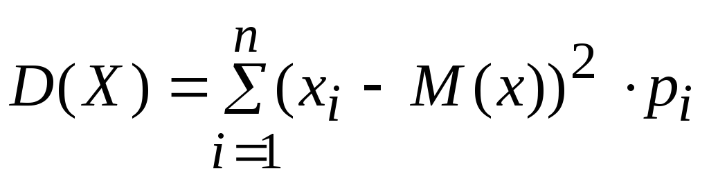
Definition: Variance D ( X ) random variable X is the mathematical expectation of the squared deviation of the random variable from its mathematical expectation:
Dispersion properties:
1)D(C)=0, where C is a constant value;
2)D(X)>0, where X is a random variable;
3)D(C X)=C2 D(X), where C is a constant value;
4)D(X+Y)=D(X)+D(Y), where X, Y are independent random variables;
To calculate variance it is often convenient to use the formula:
D(X)=M(X2)-(M(X))2,
where M(X)=∑ xi2рi= x12р1 + x22р2+…+ xn2рn
The variance D(X) has the dimension of a squared random variable, which is not always convenient. Therefore, the value √D(X) is also used as an indicator of the dispersion of possible values of a random variable.
Definition: Standard deviation σ(X) random variable X is called the square root of the variance:
![]()
Task No. 2. The discrete random variable X is specified by the distribution law:
Find P2, the distribution function F(x) and plot its graph, as well as M(X), D(X), σ(X).
Solution: Since the sum of the probabilities of possible values of the random variable X is equal to 1, then
Р2=1- (0.1+0.3+0.2+0.3)=0.1
Let's find the distribution function F(x)=P(X Geometrically, this equality can be interpreted as follows: F(x) is the probability that the random variable will take the value that is represented on the number axis by the point lying to the left of the point x. If x≤-1, then F(x)=0, since there is not a single value of this random variable on (-∞;x); If -1<х≤0, то F(х)=Р(Х=-1)=0,1, т. к. в промежуток (-∞;х) попадает только одно значение x1=-1; If 0<х≤1, то F(х)=Р(Х=-1)+ Р(Х=0)=0,1+0,1=0,2, т. к. в промежуток (-∞;x) there are two values x1=-1 and x2=0; If 1<х≤2, то F(х)=Р(Х=-1) + Р(Х=0)+ Р(Х=1)= 0,1+0,1+0,3=0,5, т. к. в промежуток (-∞;х) попадают три значения x1=-1, x2=0 и x3=1; If 2<х≤3, то F(х)=Р(Х=-1) + Р(Х=0)+ Р(Х=1)+ Р(Х=2)= 0,1+0,1+0,3+0,2=0,7, т. к. в промежуток (-∞;х) попадают четыре значения x1=-1, x2=0,x3=1 и х4=2; If x>3, then F(x)=P(X=-1) + P(X=0)+ P(X=1)+ P(X=2)+P(X=3)= 0.1 +0.1+0.3+0.2+0.3=1, because four values x1=-1, x2=0, x3=1, x4=2 fall into the interval (-∞;x) and x5=3. https://pandia.ru/text/78/455/images/image006_89.gif" width="14 height=2" height="2"> 0 at x≤-1, 0.1 at -1<х≤0, 0.2 at 0<х≤1, F(x)= 0.5 at 1<х≤2, 0.7 at 2<х≤3, 1 at x>3 Let's represent the function F(x) graphically (Fig. 3): https://pandia.ru/text/78/455/images/image014_24.jpg" width="158 height=29" height="29">≈1.2845. §
4. Binomial distribution law discrete random variable, Poisson's law. Definition: Binomial
is called the law of distribution of a discrete random variable X - the number of occurrences of event A in n independent repeated trials, in each of which event A may occur with probability p or not occur with probability q = 1-p. Then P(X=m) - the probability of occurrence of event A exactly m times in n trials is calculated using the Bernoulli formula: Р(Х=m)=Сmnpmqn-m The mathematical expectation, dispersion and standard deviation of a random variable X distributed according to a binary law are found, respectively, using the formulas: https://pandia.ru/text/78/455/images/image016_31.gif" width="26"> The probability of event A - “rolling out a five” in each trial is the same and equal to 1/6, i.e. . P(A)=p=1/6, then P(A)=1-p=q=5/6, where - “failure to get an A.” The random variable X can take the following values: 0;1;2;3. We find the probability of each of the possible values of X using Bernoulli’s formula: Р(Х=0)=Р3(0)=С03р0q3=1 (1/6)0 (5/6)3=125/216; Р(Х=1)=Р3(1)=С13р1q2=3 (1/6)1 (5/6)2=75/216; Р(Х=2)=Р3(2)=С23р2q =3 (1/6)2 (5/6)1=15/216; Р(Х=3)=Р3(3)=С33р3q0=1 (1/6)3 (5/6)0=1/216. That. the distribution law of the random variable X has the form: Control: 125/216+75/216+15/216+1/216=1. Let's find the numerical characteristics of the random variable X: M(X)=np=3 (1/6)=1/2, D(X)=npq=3 (1/6) (5/6)=5/12, Task No. 4. An automatic machine stamps parts. The probability that a manufactured part will be defective is 0.002. Find the probability that among 1000 selected parts there will be: a) 5 defective; b) at least one is defective. Solution:
The number n=1000 is large, the probability of producing a defective part p=0.002 is small, and the events under consideration (the part turns out to be defective) are independent, therefore the Poisson formula holds: Рn(m)= e-
λ
λm Let's find λ=np=1000 0.002=2. a) Find the probability that there will be 5 defective parts (m=5): Р1000(5)= e-2
25
= 32 0,13534
= 0,0361 b) Find the probability that there will be at least one defective part. Event A - “at least one of the selected parts is defective” is the opposite of the event - “all selected parts are not defective.” Therefore, P(A) = 1-P(). Hence the desired probability is equal to: P(A)=1-P1000(0)=1- e-2
20
= 1- e-2=1-0.13534≈0.865. Tasks for independent work.
1.1
1.2.
The dispersed random variable X is specified by the distribution law: Find p4, the distribution function F(X) and plot its graph, as well as M(X), D(X), σ(X). 1.3.
There are 9 markers in the box, 2 of which no longer write. Take 3 markers at random. Random variable X is the number of writing markers among those taken. Draw up a law of distribution of a random variable. 1.4.
There are 6 textbooks randomly arranged on a library shelf, 4 of which are bound. The librarian takes 4 textbooks at random. Random variable X is the number of bound textbooks among those taken. Draw up a law of distribution of a random variable. 1.5.
There are two tasks on the ticket. The probability of correctly solving the first problem is 0.9, the second is 0.7. Random variable X is the number of correctly solved problems in the ticket. Draw up a distribution law, calculate the mathematical expectation and variance of this random variable, and also find the distribution function F(x) and build its graph. 1.6.
Three shooters are shooting at a target. The probability of hitting the target with one shot is 0.5 for the first shooter, 0.8 for the second, and 0.7 for the third. Random variable X is the number of hits on the target if the shooters fire one shot at a time. Find the distribution law, M(X),D(X). 1.7.
A basketball player throws the ball into the basket with a probability of hitting each shot of 0.8. For each hit, he receives 10 points, and if he misses, no points are awarded to him. Draw up a distribution law for the random variable X - the number of points received by a basketball player in 3 shots. Find M(X),D(X), as well as the probability that he gets more than 10 points. 1.8.
Letters are written on the cards, a total of 5 vowels and 3 consonants. 3 cards are chosen at random, and each time the taken card is returned back. Random variable X is the number of vowels among those taken. Draw up a distribution law and find M(X),D(X),σ(X). 1.9.
On average, under 60% of contracts, the insurance company pays insurance amounts in connection with the occurrence of an insured event. Draw up a distribution law for the random variable X - the number of contracts for which the insurance amount was paid among four contracts selected at random. Find the numerical characteristics of this quantity. 1.10.
The radio station sends call signs (no more than four) at certain intervals until two-way communication is established. The probability of receiving a response to a call sign is 0.3. Random variable X is the number of call signs sent. Draw up a distribution law and find F(x). 1.11.
There are 3 keys, of which only one fits the lock. Draw up a law for the distribution of the random variable X-number of attempts to open the lock, if the tried key does not participate in subsequent attempts. Find M(X),D(X). 1.12.
Consecutive independent tests of three devices are carried out for reliability. Each subsequent device is tested only if the previous one turned out to be reliable. The probability of passing the test for each device is 0.9. Draw up a distribution law for the random variable X-number of tested devices. 1.13
.Discrete random variable X has three possible values: x1=1, x2, x3, and x1<х2<х3. Вероятность того, что Х примет значения х1 и х2, соответственно равны 0,3 и 0,2. Известно, что М(Х)=2,2, D(X)=0,76. Составить закон распределения случайной величины. 1.14.
The electronic device block contains 100 identical elements. The probability of failure of each element during time T is 0.002. The elements work independently. Find the probability that no more than two elements will fail during time T. 1.15.
The textbook was published in a circulation of 50,000 copies. The probability that the textbook is bound incorrectly is 0.0002. Find the probability that the circulation contains: a) four defective books, b) less than two defective books. 1
.16.
The number of calls arriving at the PBX every minute is distributed according to Poisson's law with the parameter λ=1.5. Find the probability that in a minute the following will arrive: a) two calls; b) at least one call. 1.17.
Find M(Z),D(Z) if Z=3X+Y. 1.18.
The laws of distribution of two independent random variables are given: Find M(Z),D(Z) if Z=X+2Y. Answers:
https://pandia.ru/text/78/455/images/image007_76.gif" height="110"> 1.1.
p3=0.4; 0 at x≤-2, 0.3 at -2<х≤0, F(x)= 0.5 at 0<х≤2, 0.9 at 2<х≤5, 1 at x>5 0.3 at -1<х≤0, 0.4 at 0<х≤1, F(x)= 0.6 at 1<х≤2, 0.7 at 2<х≤3, 1 at x>3 M(X)=1; D(X)=2.6; σ(X) ≈1.612. https://pandia.ru/text/78/455/images/image025_24.gif" width="2 height=98" height="98"> 0 at x≤0, 0.03 at 0<х≤1, F(x)= 0.37 at 1<х≤2, 1 for x>2 M(X)=2; D(X)=0.62 M(X)=2.4; D(X)=0.48, P(X>10)=0.896 1.
8
.
M(X)=15/8; D(X)=45/64; σ(X) ≈ M(X)=2.4; D(X)=0.96 https://pandia.ru/text/78/455/images/image008_71.gif" width="14"> 1.11.
M(X)=2; D(X)=2/3 1.14.
1.22 e-0.2≈0.999 1.15.
a)0.0189; b) 0.00049 1.16.
a)0.0702; b)0.77687 1.17.
3,8; 14,2 1.18.
11,2; 4. Chapter 2. Continuous random variable
Definition: Continuous
is a quantity whose all possible values completely fill a finite or infinite span of the number line. Obviously, the number of possible values of a continuous random variable is infinite. A continuous random variable can be specified using a distribution function. Definition: F distribution function
a continuous random variable X is called a function F(x), which determines for each value xhttps://pandia.ru/text/78/455/images/image028_11.jpg" width="14" height="13">R The distribution function is sometimes called the cumulative distribution function. Properties of the distribution function:
1)1≤ F(x) ≤1 2) For a continuous random variable, the distribution function is continuous at any point and differentiable everywhere, except, perhaps, at individual points. 3) The probability of a random variable X falling into one of the intervals (a;b), [a;b], [a;b], is equal to the difference between the values of the function F(x) at points a and b, i.e. R(a)<Х 4) The probability that a continuous random variable X will take one separate value is 0. 5) F(-∞)=0, F(+∞)=1 Specifying a continuous random variable using a distribution function is not the only way. Let us introduce the concept of probability distribution density (distribution density). Definition
:
Probability distribution density
f
(
x
)
of a continuous random variable X is the derivative of its distribution function, i.e.: The probability density function is sometimes called the differential distribution function or differential distribution law. The graph of the probability density distribution f(x) is called probability distribution curve
.
Properties of probability density distribution:
1) f(x) ≥0, at xhttps://pandia.ru/text/78/455/images/image029_10.jpg" width="285" height="141">DIV_ADBLOCK92"> https://pandia.ru/text/78/455/images/image032_23.gif" height="38 src="> +∞ 2 6 +∞ 6 6 ∫ f(x)dx=∫ 0dx+ ∫ c(x-2)dx +∫ 0dx= c∫ (x-2)dx=c(x2/2-2x) =c(36/2-12-(4/ 2-4))=8s; b) It is known that F(x)= ∫ f(x)dx Therefore, x if x≤2, then F(x)= ∫ 0dx=0; https://pandia.ru/text/78/455/images/image032_23.gif" height="38 src="> 2 6 x 6 6 if x>6, then F(x)= ∫ 0dx+∫ 1/8(x-2)dx+∫ 0dx=1/8∫(x-2)dx=1/8(x2/2-2x) = 1/8(36/2-12-(4/2+4))=1/8 8=1. Thus, 0 at x≤2, F(x)= (x-2)2/16 at 2<х≤6, 1 for x>6. The graph of the function F(x) is shown in Fig. 3 https://pandia.ru/text/78/455/images/image034_23.gif" width="14" height="62 src="> 0 at x≤0, F(x)= (3 arctan x)/π at 0<х≤√3, 1 for x>√3. Find the differential distribution function f(x) Solution:
Since f(x)= F’(x), then DIV_ADBLOCK93"> · Mathematical expectation M (X)
continuous random variable X are determined by the equality: M(X)= ∫ x f(x)dx, provided that this integral converges absolutely. · Dispersion
D
(
X
)
continuous random variable X is determined by the equality: D(X)= ∫ (x-M(x)2) f(x)dx, or D(X)= ∫ x2 f(x)dx - (M(x))2 · Standard deviation σ(X)
continuous random variable is determined by the equality: All properties of mathematical expectation and dispersion, discussed earlier for dispersed random variables, are also valid for continuous ones. Task No. 3. The random variable X is specified by the differential function f(x): https://pandia.ru/text/78/455/images/image036_19.gif" height="38"> -∞ 2 X3/9 + x2/6 = 8/9-0+9/6-4/6=31/18, https://pandia.ru/text/78/455/images/image032_23.gif" height="38"> +∞ D(X)= ∫ x2 f(x)dx-(M(x))2=∫ x2 x/3 dx+∫1/3x2 dx=(31/18)2=x4/12 + x3/9 - - (31/18)2=16/12-0+27/9-8/9-(31/18)2=31/9- (31/18)2==31/9(1-31/36)=155/324, https://pandia.ru/text/78/455/images/image032_23.gif" height="38"> P(1<х<5)= ∫ f(x)dx=∫ х/3 dx+∫ 1/3 dx+∫ 0 dx= х2/6 +1/3х = 4/6-1/6+1-2/3=5/6. Problems for independent solution.
2.1.
A continuous random variable X is specified by the distribution function: 0 at x≤0, F(x)= https://pandia.ru/text/78/455/images/image038_17.gif" width="14" height="86"> 0 for x≤ π/6, F(x)= - cos 3x at π/6<х≤ π/3, 1 for x> π/3. Find the differential distribution function f(x), and also Р(2π /9<Х< π /2). 2.3.
0 at x≤2, f(x)= c x at 2<х≤4, 0 for x>4. 2.4.
A continuous random variable X is specified by the distribution density: 0 at x≤0, f(x)= c √x at 0<х≤1, 0 for x>1. Find: a) number c; b) M(X), D(X). 2.5.
https://pandia.ru/text/78/455/images/image041_3.jpg" width="36" height="39"> at x, 0 at x. Find: a) F(x) and construct its graph; b) M(X),D(X), σ(X); c) the probability that in four independent trials the value of X will take exactly 2 times the value belonging to the interval (1;4). 2.6.
The probability distribution density of a continuous random variable X is given: f(x)= 2(x-2) at x, 0 at x. Find: a) F(x) and construct its graph; b) M(X),D(X), σ (X); c) the probability that in three independent trials the value of X will take exactly 2 times the value belonging to the segment . 2.7.
The function f(x) is given as: https://pandia.ru/text/78/455/images/image045_4.jpg" width="43" height="38 src=">.jpg" width="16" height="15">[-√ 3/2; √3/2]. 2.8.
The function f(x) is given as: https://pandia.ru/text/78/455/images/image046_5.jpg" width="45" height="36 src="> .jpg" width="16" height="15">[- π /4 ; π /4]. Find: a) the value of the constant c at which the function will be the probability density of some random variable X; b) distribution function F(x). 2.9.
The random variable X, concentrated on the interval (3;7), is specified by the distribution function F(x)= . Find the probability that random variable X will take the value: a) less than 5, b) not less than 7. 2.10.
Random variable X, concentrated on the interval (-1;4), is given by the distribution function F(x)= . Find the probability that random variable X will take the value: a) less than 2, b) not less than 4. 2.11.
https://pandia.ru/text/78/455/images/image049_6.jpg" width="43" height="44 src="> .jpg" width="16" height="15">. Find: a) number c; b) M(X); c) probability P(X> M(X)). 2.12.
The random variable is specified by the differential distribution function: https://pandia.ru/text/78/455/images/image050_3.jpg" width="60" height="38 src=">.jpg" width="16 height=15" height="15"> . Find: a) M(X); b) probability P(X≤M(X)) 2.13.
The Rem distribution is given by the probability density: https://pandia.ru/text/78/455/images/image052_5.jpg" width="46" height="37"> for x ≥0. Prove that f(x) is indeed a probability density function. 2.14.
The probability distribution density of a continuous random variable X is given: DIV_ADBLOCK96"> https://pandia.ru/text/78/455/images/image055_3.jpg" width="187 height=136" height="136">(Fig. 5) 2.16.
The random variable X is distributed according to the “right triangle” law in the interval (0;4) (Fig. 5). Find an analytical expression for the probability density f(x) on the entire number line. Answers
0 at x≤0, f(x)= https://pandia.ru/text/78/455/images/image038_17.gif" width="14" height="86"> 0 for x≤ π/6, F(x)= 3sin 3x at π/6<х≤ π/3,
Непрерывная случайная величина Х имеет равномерный закон распределения на некотором интервале (а;b), которому принадлежат все возможные значения Х, если плотность распределения вероятностей f(x) постоянная на этом интервале и равна 0 вне его, т. е. 0 for x≤a, f(x)= for a<х 0 for x≥b. The graph of the function f(x) is shown in Fig. 1 F(x)= https://pandia.ru/text/78/455/images/image077_3.jpg" width="30" height="37">, D(X)=, σ(X)=. Task No. 1. The random variable X is uniformly distributed on the segment. Find: a) probability distribution density f(x) and plot it; b) the distribution function F(x) and plot it; c) M(X),D(X), σ(X). Solution:
Using the formulas discussed above, with a=3, b=7, we find: https://pandia.ru/text/78/455/images/image081_2.jpg" width="22" height="39"> at 3≤х≤7, 0 for x>7 Let's build its graph (Fig. 3): https://pandia.ru/text/78/455/images/image038_17.gif" width="14" height="86 src="> 0 at x≤3, F(x)= https://pandia.ru/text/78/455/images/image084_3.jpg" width="203" height="119 src=">Fig. 4 D(X) = ==https://pandia.ru/text/78/455/images/image089_1.jpg" width="37" height="43">==https://pandia.ru/text/ 78/455/images/image092_10.gif" width="14" height="49 src="> 0 at x<0, f(x)= λе-λх for x≥0. The distribution function of a random variable X, distributed according to the exponential law, is given by the formula: DIV_ADBLOCK98"> https://pandia.ru/text/78/455/images/image095_4.jpg" width="161" height="119 src="> Fig. 6 The mathematical expectation, variance and standard deviation of the exponential distribution are respectively equal to: M(X)= , D(X)=, σ (Х)= Thus, the mathematical expectation and the standard deviation of the exponential distribution are equal to each other. The probability of X falling into the interval (a;b) is calculated by the formula: P(a<Х Task No. 2. The average failure-free operation time of the device is 100 hours. Assuming that the failure-free operation time of the device has an exponential distribution law, find: a) probability distribution density; b) distribution function; c) the probability that the device’s failure-free operation time will exceed 120 hours. Solution:
According to the condition, the mathematical distribution M(X)=https://pandia.ru/text/78/455/images/image098_10.gif" height="43 src="> 0 at x<0, a) f(x)= 0.01e -0.01x for x≥0. b) F(x)= 0 at x<0, 1-e -0.01x at x≥0. c) We find the desired probability using the distribution function: P(X>120)=1-F(120)=1-(1- e -1.2)= e -1.2≈0.3. §
3.Normal distribution law Definition:
A continuous random variable X has normal distribution law (Gauss's law),
if its distribution density has the form: where m=M(X), σ2=D(X), σ>0. The normal distribution curve is called normal or Gaussian curve
(Fig.7) The distribution function of a random variable X, distributed according to the normal law, is expressed through the Laplace function Ф (x) according to the formula: where is the Laplace function. Comment:
The function Ф(x) is odd (Ф(-х)=-Ф(х)), in addition, for x>5 we can assume Ф(х) ≈1/2. The graph of the distribution function F(x) is shown in Fig. 8 https://pandia.ru/text/78/455/images/image106_4.jpg" width="218" height="33"> The probability that the absolute value of the deviation is less than a positive number δ is calculated by the formula: In particular, for m=0 the following equality holds: "Three Sigma Rule"
If a random variable X has a normal distribution law with parameters m and σ, then it is almost certain that its value lies in the interval (a-3σ; a+3σ), because https://pandia.ru/text/78/455/images/image110_2.jpg" width="157" height="57 src=">a) b) Let's use the formula: https://pandia.ru/text/78/455/images/image112_2.jpg" width="369" height="38 src="> From the table of function values Ф(х) we find Ф(1.5)=0.4332, Ф(1)=0.3413. So, the desired probability: P(28 Tasks for independent work
3.1.
The random variable X is uniformly distributed in the interval (-3;5). Find: b) distribution function F(x); c) numerical characteristics; d) probability P(4<х<6). 3.2.
The random variable X is uniformly distributed on the segment. Find: a) distribution density f(x); b) distribution function F(x); c) numerical characteristics; d) probability P(3≤х≤6). 3.3.
There is an automatic traffic light on the highway, in which the green light is on for 2 minutes, yellow for 3 seconds, red for 30 seconds, etc. A car drives along the highway at a random moment in time. Find the probability that a car will pass a traffic light without stopping. 3.4.
Subway trains run regularly at intervals of 2 minutes. A passenger enters the platform at a random time. What is the probability that a passenger will have to wait more than 50 seconds for a train? Find the mathematical expectation of the random variable X - the waiting time for the train. 3.5.
Find the variance and standard deviation of the exponential distribution given by the distribution function: F(x)= 0 at x<0, 1st-8x for x≥0. 3.6.
A continuous random variable X is specified by the probability distribution density: f(x)= 0 at x<0, 0.7 e-0.7x at x≥0. a) Name the distribution law of the random variable under consideration. b) Find the distribution function F(X) and the numerical characteristics of the random variable X. 3.7.
The random variable X is distributed according to the exponential law specified by the probability distribution density: f(x)= 0 at x<0, 0.4 e-0.4 x at x≥0. Find the probability that as a result of the test X will take a value from the interval (2.5;5). 3.8.
A continuous random variable X is distributed according to the exponential law specified by the distribution function: F(x)= 0 at x<0, 1st-0.6x at x≥0 Find the probability that, as a result of the test, X will take a value from the segment. 3.9.
The expected value and standard deviation of a normally distributed random variable are 8 and 2, respectively. Find: a) distribution density f(x); b) the probability that as a result of the test X will take a value from the interval (10;14). 3.10.
The random variable X is normally distributed with a mathematical expectation of 3.5 and a variance of 0.04. Find: a) distribution density f(x); b) the probability that as a result of the test X will take a value from the segment . 3.11.
The random variable X is normally distributed with M(X)=0 and D(X)=1. Which of the events: |X|≤0.6 or |X|≥0.6 is more likely? 3.12.
The random variable X is distributed normally with M(X)=0 and D(X)=1. From which interval (-0.5;-0.1) or (1;2) is it more likely to take a value during one test? 3.13.
The current price per share can be modeled using the normal distribution law with M(X)=10 den. units and σ (X)=0.3 den. units Find: a) the probability that the current share price will be from 9.8 den. units up to 10.4 days units; b) using the “three sigma rule”, find the boundaries within which the current stock price will be located. 3.14.
The substance is weighed without systematic errors. Random weighing errors are subject to the normal law with the mean square ratio σ=5g. Find the probability that in four independent experiments an error in three weighings will not occur in absolute value 3r. 3.15.
The random variable X is normally distributed with M(X)=12.6. The probability of a random variable falling into the interval (11.4;13.8) is 0.6826. Find the standard deviation σ. 3.16.
The random variable X is distributed normally with M(X)=12 and D(X)=36. Find the interval into which the random variable X will fall as a result of the test with a probability of 0.9973. 3.17.
A part manufactured by an automatic machine is considered defective if the deviation X of its controlled parameter from the nominal value exceeds modulo 2 units of measurement. It is assumed that the random variable X is normally distributed with M(X)=0 and σ(X)=0.7. What percentage of defective parts does the machine produce? 3.18.
The X parameter of the part is distributed normally with a mathematical expectation of 2 equal to the nominal value and a standard deviation of 0.014. Find the probability that the deviation of X from the nominal value will not exceed 1% of the nominal value. Answers
https://pandia.ru/text/78/455/images/image116_9.gif" width="14" height="110 src="> b) 0 for x≤-3, F(x)= left"> 3.10.
a)f(x)= , b) Р(3.1≤Х≤3.7) ≈0.8185. 3.11.
|x|≥0.6. 3.12.
(-0,5;-0,1). 3.13.
a) P(9.8≤Х≤10.4) ≈0.6562. 3.14.
0,111. 3.15.
σ=1.2. 3.16.
(-6;30). 3.17.
0,4%. X; meaning F(5); the probability that the random variable X will take values from the segment . Construct a distribution polygon. Set the law of distribution of a random variable X in the form of a table. Find the distribution function of a random variable X. Construct graphs of functions and . Calculate the mathematical expectation, variance, mode and median of a random variable X. Sample A: 6 9 7 6 4 4 Sample B: 55 72 54 53 64 53 59 48 42 46 50 63 71 56 54 59 54 44 50 43 51 52 60 43 50 70 68 59 53 58 62 49 59 51 52 47 57 71 60 46 55 58 72 47 60 65 63 63 58 56 55 51 64 54 54 63 56 44 73 41 68 54 48 52 52 50 55 49 71 67 58 46 50 51 72 63 64 48 47 55 Option 17. Calculate its mathematical expectation and variance. Find the distribution function of a random variable X. Construct graphs of functions and . Calculate the mathematical expectation, variance, mode and median of the random variable X. · sample average; · sample variance; Mode and median; Sample A: 0 0 2 2 1 4 · sample average; · sample variance; standard sample deviation; · mode and median; Sample B: 166 154 168 169 178 182 169 159 161 150 149 173 173 156 164 169 157 148 169 149 157 171 154 152 164 157 177 155 167 169 175 166 167 150 156 162 170 167 161 158 168 164 170 172 173 157 157 162 156 150 154 163 143 170 170 168 151 174 155 163 166 173 162 182 166 163 170 173 159 149 172 176 Option 18. Calculate its mathematical expectation and variance. Find the distribution function of the random variable X. Draw graphs of the functions and . Calculate the mathematical expectation, variance, mode and median of a random variable X. · sample average; · sample variance; standard sample deviation; · mode and median; Sample A: 4 7 6 3 3 4 · sample average; · sample variance; standard sample deviation; · mode and median; Sample B: 152 161 141 155 171 160 150 157 154 164 138 172 155 152 177 160 168 157 115 128 154 149 150 141 172 154 144 177 151 128 150 147 143 164 156 145 156 170 171 142 148 153 152 170 142 153 162 128 150 146 155 154 163 142 171 138 128 158 140 160 144 150 162 151 163 157 177 127 141 160 160 142 159 147 142 122 155 144 170 177 Option 19. 1. There are 16 women and 5 men working at the site. 3 people were selected at random using their personnel numbers. Find the probability that all selected people will be men. 2. Four coins are tossed. Find the probability that only two coins will have a “coat of arms”. 3. The word “PSYCHOLOGY” is made up of cards, each of which has one letter written on it. The cards are shuffled and taken out one at a time without returning. Find the probability that the letters taken out form a word: a) PSYCHOLOGY; b) STAFF. 4. The urn contains 6 black and 7 white balls. 5 balls are randomly drawn. Find the probability that among them there are: a. 3 white balls; b. less than 3 white balls; c. at least one white ball. 5. Probability of an event occurring A in one trial is equal to 0.5. Find the probabilities of the following events: a. event A appears 3 times in a series of 5 independent trials; b. event A will appear at least 30 and no more than 40 times in a series of 50 trials. 6. There are 100 machines of the same power, operating independently of each other in the same mode, in which their drive is turned on for 0.8 working hours. What is the probability that at any given moment in time from 70 to 86 machines will be turned on? 7. The first urn contains 4 white and 7 black balls, and the second urn contains 8 white and 3 black balls. 4 balls are randomly drawn from the first urn, and 1 ball from the second. Find the probability that among the drawn balls there are only 4 black balls. 8. The car sales showroom receives cars of three brands daily in volumes: “Moskvich” – 40%; "Oka" - 20%; "Volga" - 40% of all imported cars. Among Moskvich cars, 0.5% have an anti-theft device, Oka – 0.01%, Volga – 0.1%. Find the probability that the car taken for inspection has an anti-theft device. 9. Numbers and are chosen at random on the segment. Find the probability that these numbers satisfy the inequalities. 10. The law of distribution of a random variable is given X: Find the distribution function of a random variable X; meaning F(2); the probability that the random variable X will take values from the interval . Construct a distribution polygon. In applications of probability theory, the quantitative characteristics of the experiment are of primary importance. A quantity that can be quantitatively determined and which, as a result of an experiment, can take on different values depending on the case is called random variable. Examples of random variables: 1. The number of times an even number of points appears in ten throws of a die. 2. The number of hits on the target by a shooter who fires a series of shots. 3. The number of fragments of an exploding shell. In each of the examples given, the random variable can only take on isolated values, that is, values that can be numbered using a natural series of numbers. Such a random variable, the possible values of which are individual isolated numbers, which this variable takes with certain probabilities, is called discrete. The number of possible values of a discrete random variable can be finite or infinite (countable). Law of distribution A discrete random variable is a list of its possible values and their corresponding probabilities. The distribution law of a discrete random variable can be specified in the form of a table (probability distribution series), analytically and graphically (probability distribution polygon). When carrying out an experiment, it becomes necessary to evaluate the value being studied “on average.” The role of the average value of a random variable is played by a numerical characteristic called mathematical expectation, which is determined by the formula Where x 1 , x 2
,.. , x n– random variable values X, A p 1 ,p 2 ,
... , p n– the probabilities of these values (note that p 1
+
p 2
+…+
p n =
1). Example. Shooting is carried out at the target (Fig. 11). A hit in I gives three points, in II – two points, in III – one point. The number of points scored in one shot by one shooter has a distribution law of the form To compare the skill of shooters, it is enough to compare the average values of the points scored, i.e. mathematical expectations M(X) And M(Y):
M(X)
=
1
0,4
+ 2
0,2
+ 3
0,4
= 2,0, M(Y)
=
1
0,2
+ 2
0,5
+ 3
0,3
= 2,1. The second shooter gives on average a slightly higher number of points, i.e. it will give better results when fired repeatedly. Let us note the properties of the mathematical expectation: 1. The mathematical expectation of a constant value is equal to the constant itself: M(C)
= C. 2. The mathematical expectation of the sum of random variables is equal to the sum of the mathematical expectations of the terms: M =(X 1 +
X 2 +…+
X n)=
M(X 1)+
M(X 2)+…+
M(X n). 3. The mathematical expectation of the product of mutually independent random variables is equal to the product of the mathematical expectations of the factors M(X 1 X 2 …
X n)
=
M(X 1)M(X 2)…
M(X n). 4. The mathematical negation of the binomial distribution is equal to the product of the number of trials and the probability of an event occurring in one trial (task 4.6). M(X)
= pr. To assess how a random variable “on average” deviates from its mathematical expectation, i.e. In order to characterize the spread of values of a random variable in probability theory, the concept of dispersion is used. Variance random variable X is called the mathematical expectation of the squared deviation: D(X)
=
M[(X
-
M(X)) 2 ]. Dispersion is a numerical characteristic of the dispersion of a random variable. From the definition it is clear that the smaller the dispersion of a random variable, the more closely its possible values are located around the mathematical expectation, that is, the better the values of the random variable are characterized by its mathematical expectation. From the definition it follows that the variance can be calculated using the formula It is convenient to calculate the variance using another formula: D(X)
=
M(X 2)
- (M(X)) 2 .
The dispersion has the following properties: 1. The variance of the constant is zero: D(C)
=
0.
2. The constant factor can be taken out of the dispersion sign by squaring it: D(CX)
=
C 2 D(X). 3. The variance of the sum of independent random variables is equal to the sum of the variance of the terms: D(X 1 +
X 2 +
X 3 +…+
X n)=
D(X 1)+
D(X 2)+…+
D(X n) 4. The variance of the binomial distribution is equal to the product of the number of trials and the probability of the occurrence and non-occurrence of an event in one trial: D(X)
= npq. In probability theory, a numerical characteristic equal to the square root of the variance of a random variable is often used. This numerical characteristic is called the mean square deviation and is denoted by the symbol It characterizes the approximate size of the deviation of a random variable from its average value and has the same dimension as the random variable. 4.1.
The shooter fires three shots at the target. The probability of hitting the target with each shot is 0.3. Construct a distribution series for the number of hits. Solution. The number of hits is a discrete random variable X. Each value x n
random variable X corresponds to a certain probability P n . The distribution law of a discrete random variable in this case can be specified near distribution. In this problem X takes values 0, 1, 2, 3. According to Bernoulli's formula Let's find the probabilities of possible values of the random variable: R 3 (0)
= (0,7) 3 =
0,343, R 3 (1)
= R 3 (2)
= R 3 (3)
= (0,3) 3 =
0,027. By arranging the values of the random variable X in increasing order, we obtain the distribution series: X n Note that the amount means the probability that the random variable X will take at least one value from among the possible ones, and this event is reliable, therefore 4.2
.There are four balls in the urn with numbers from 1 to 4. Two balls are taken out. Random value X– the sum of the ball numbers. Construct a distribution series of a random variable X. Solution. Random variable values X are 3, 4, 5, 6, 7. Let's find the corresponding probabilities. Random variable value 3 X can be accepted in the only case when one of the selected balls has the number 1, and the other 2. The number of possible test outcomes is equal to the number of combinations of four (the number of possible pairs of balls) of two. Using the classical probability formula we get Likewise, R(X= 4) =R(X= 6) =R(X= 7) = 1/6. The sum 5 can appear in two cases: 1 + 4 and 2 + 3, so X has the form: Find the distribution function F(x) random variable X and plot it. Calculate for X its mathematical expectation and variance. Solution. The distribution law of a random variable can be specified by the distribution function F(x)
= P(X
x).
Distribution function F(x) is a non-decreasing, left-continuous function defined on the entire number line, while F
(-
)=
0,F
(+
)=
1. For a discrete random variable, this function is expressed by the formula Therefore in this case Distribution function graph F(x) is a stepped line (Fig. 12) F(x) Expected valueM(X) is the weighted arithmetic average of the values X 1 , X 2 ,……X n random variable X with scales ρ
1,
ρ
2, ……
, ρ
n
and is called the mean value of the random variable X. According to the formula M(X)= x 1
ρ
1 + x 2
ρ
2 +……+ x n
ρ
n M(X) = 3·0.14+5·0.2+7·0.49+11·0.17 = 6.72. Dispersion characterizes the degree of dispersion of the values of a random variable from its average value and is denoted D(X): D(X)=M[(HM(X)) 2 ]= M(X 2)
–[M(X)] 2 . For a discrete random variable, the variance has the form or it can be calculated using the formula Substituting the numerical data of the problem into the formula, we get: M(X 2)
=
3 2
∙ 0,14+5 2
∙ 0,2+7 2
∙ 0,49+11 2
∙ 0,17 = 50,84 D(X)
= 50,84-6,72 2
= 5,6816. 4.4.
Two dice are rolled twice at the same time. Write the binomial law of distribution of a discrete random variable X- the number of occurrences of an even total number of points on two dice. Solution. Let us introduce a random event A= (two dice with one throw resulted in a total of even number of points). Using the classical definition of probability we find R(A)=
Where n
- the number of possible test outcomes is found according to the rule multiplication: n
= 6∙6 =36, m
-
number of people favoring the event A outcomes - equal m= 3∙6=18. Thus, the probability of success in one trial is ρ
= P(A)=
1/2.
The problem is solved using a Bernoulli test scheme. One challenge here would be to roll two dice once. Number of such tests n
= 2. Random variable X takes values 0, 1, 2 with probabilities R 2 (0)
= The required binomial distribution of a random variable X can be represented as a distribution series: X n ρ
n 4.5
. In a batch of six parts there are four standard parts. Three parts were selected at random. Construct a probability distribution of a discrete random variable X– the number of standard parts among those selected and find its mathematical expectation. Solution. Random variable values X are the numbers 0,1,2,3. It's clear that R(X=0)=0, since there are only two non-standard parts. R(X=1) = R(X= 2) = R(X=3) = Distribution law of a random variable X Let's present it in the form of a distribution series: X n ρ
n Expected value M(X)=1
∙ 1/5+2 ∙ 3/5+3 ∙ 1/5=2. 4.6
. Prove that the mathematical expectation of a discrete random variable X- number of occurrences of the event A V n independent trials, in each of which the probability of an event occurring is equal to ρ
– equal to the product of the number of trials by the probability of the occurrence of an event in one trial, that is, to prove that the mathematical expectation of the binomial distribution M(X)
=n .
ρ
, and dispersion D(X)
=n.p.
. Solution. Random value X can take values 0, 1, 2..., n. Probability R(X= k) is found using Bernoulli’s formula: R(X=k)= R n(k)= Distribution series of a random variable X has the form: X n ρ
n q n Where q=
1-
ρ
. For the mathematical expectation we have the expression: M(X)= In the case of one test, that is, with n= 1 for random variable X 1 – number of occurrences of the event A- the distribution series has the form: X n ρ
n M(X 1)=
0∙q +
1
∙ p
=
p D(X 1)
=
p
–
p 2
=
p(1-
p)
=
pq. If X k – number of occurrences of the event A in which test, then R(X To)=
ρ
And X=X 1 +X 2 +….+X n . From here we get M(X)=M(X 1
)+M(X 2)+
… +M(X n)=
nρ,
D(X)=D(X 1)+D(X 2)+
...
+D(X n)=npq. 4.7.
The quality control department checks products for standardness. The probability that the product is standard is 0.9. Each batch contains 5 products. Find the mathematical expectation of a discrete random variable X- the number of batches, each of which will contain 4 standard products - if 50 batches are subject to inspection. Solution. The probability that there will be 4 standard products in each randomly selected batch is constant; let's denote it by ρ
.Then the mathematical expectation of the random variable X equals M(X)=
50∙ρ.
Let's find the probability ρ
according to Bernoulli's formula: ρ=P 5 (4)= M(X)=
50∙0,32=16. 4.8
. Three dice are thrown. Find the mathematical expectation of the sum of the dropped points. Solution. You can find the distribution of a random variable X- the sum of the dropped points and then its mathematical expectation. However, this path is too cumbersome. It is easier to use another technique, representing a random variable X, the mathematical expectation of which needs to be calculated, in the form of a sum of several simpler random variables, the mathematical expectation of which is easier to calculate. If the random variable X i is the number of points rolled on i– th bones ( i= 1, 2, 3), then the sum of points X will be expressed in the form X = X 1 + X 2 + X 3 . To calculate the mathematical expectation of the original random variable, all that remains is to use the property of mathematical expectation M(X 1
+ X 2 + X 3
)= M(X 1
)+ M(X 2)+ M(X 3
). It's obvious that R(X i = K)=
1/6, TO=
1, 2, 3, 4, 5, 6,
i=
1,
2, 3. Therefore, the mathematical expectation of the random variable X i looks like M(X i)
=
1/6∙1
+ 1/6∙2
+1/6∙3
+ 1/6∙4
+ 1/6∙5
+ 1/6∙6
= 7/2, M(X)
=
3∙7/2 = 10,5.
4.9.
Determine the mathematical expectation of the number of devices that failed during testing if: a) the probability of failure for all devices is the same R, and the number of devices under test is equal to n; b) probability of failure for i
–
of the device is equal to p i
,
i=
1,
2, … , n. Solution. Let the random variable X is the number of failed devices, then X = X 1 + X 2 + … + X n ,
X i
=
It's clear that R(X i =
1)=
R i ,
R(X i =
0)=
1–
R i ,i= 1,
2,
…
,n. M(X i)=
1∙R i +
0∙(1-R i)=P i , M(X)=M(X 1)+M(X 2)+ … +M(X n)=P 1 +P 2 + … + P n .
In case “a” the probability of device failure is the same, that is R i =p,i= 1,
2, …
,n. M(X)=
n.p.. This answer could be obtained immediately if we notice that the random variable X has a binomial distribution with parameters ( n,
p).
4.10.
Two dice are thrown simultaneously twice. Write the binomial law of distribution of a discrete random variable X - the number of rolls of an even number of points on two dice. Solution. Let A=(rolling an even number on the first die), B =(rolling an even number on the second dice). Getting an even number on both dice in one throw is expressed by the product AB. Then R
(AB)
= R(A)∙R(IN)
=
The result of the second throw of two dice does not depend on the first, so Bernoulli's formula applies when n
=
2,p = 1/4,
q
=
1– p = 3/4.
Random value X can take values 0, 1, 2 ,
the probability of which can be found using Bernoulli’s formula: R(X= 0)= P 2
(0)
=
q
2
= 9/16, R(X= 1)= P 2
(1)= C R(X= 2)= P 2
(2)= C Distribution series of a random variable X: 4.11.
The device consists of a large number of independently operating elements with the same very small probability of failure of each element over time t. Find the average number of refusals over time t elements, if the probability that at least one element will fail during this time is 0.98. Solution.
Number of people who refused over time t elements – random variable X, which is distributed according to Poisson's law, since the number of elements is large, the elements work independently and the probability of failure of each element is small. Average number of occurrences of an event in n tests equals M(X)
=
n.p..
Since the probability of failure TO elements from n expressed by the formula R n
(TO)
where
=
n.p., then the probability that not a single element will fail during the time t
we get at K = 0: R n
(0)= e - . Therefore, the probability of the opposite event is in time t
at least one element fails – equal to 1 - e -
. According to the conditions of the problem, this probability is 0.98. From Eq. 1
- e -
= 0,98, e -
= 1 – 0,98 =
0,02, from here
=
-ln
0,02
4. So, in time t operation of the device, on average 4 elements will fail. 4.12
. The dice are rolled until a “two” comes up. Find the average number of throws. Solution. Let's introduce a random variable X– the number of tests that must be performed until the event of interest to us occurs. The probability that X= 1 is equal to the probability that during one throw of the dice a “two” will appear, i.e. R(X= 1)
= 1/6. Event X= 2 means that on the first test the “two” did not come up, but on the second it did. Probability of event X= 2 is found by the rule of multiplying the probabilities of independent events: R(X= 2)
= (5/6)∙(1/6) Likewise, R(X= 3)
= (5/6) 2 ∙1/6, R(X= 4)
= (5/6) 2 ∙1/6 etc. We obtain a series of probability distributions: (5/6) To
∙1/6 The average number of throws (trials) is the mathematical expectation M(X)
=
1∙1/6 +
2∙5/6∙1/6 + 3∙(5/6) 2 ∙1/6
+ … + TO
(5/6) TO -1 ∙1/6
+ … = 1/6∙(1+2∙5/6 +3∙(5/6) 2
+ … + TO
(5/6) TO -1
+ …) Let's find the sum of the series: Hence, M(X)
=
(1/6) (1/ (1 –
5/6) 2
= 6. Thus, you need to make an average of 6 throws of the dice until a “two” comes up. 4.13.
Independent tests are carried out with the same probability of occurrence of the event A in every test. Find the probability of an event occurring A, if the variance of the number of occurrences of an event in three independent trials is 0.63 .
Solution. The number of occurrences of an event in three trials is a random variable X, distributed according to the binomial law. The variance of the number of occurrences of an event in independent trials (with the same probability of occurrence of the event in each trial) is equal to the product of the number of trials by the probabilities of the occurrence and non-occurrence of the event (problem 4.6) D(X)
=
npq.
By condition n
=
3,
D(X)
=
0.63, so you can R find from equation 0,63
= 3∙R(1-R), which has two solutions R 1
=
0.7 and R 2
=
0,3.

 1.2.
p4=0.1; 0 at x≤-1,
1.2.
p4=0.1; 0 at x≤-1,

![]()
 https://pandia.ru/text/78/455/images/image038_17.gif" width="14" height="86"> 0 for x≤a,
 ,
, The normal curve is symmetrical with respect to the straight line x=m, has a maximum at x=a, equal to .
![]() ,
,![]()
![]()

X
–28
–20
–12
–4
p
0,22
0,44
0,17
0,1
0,07
X
p
0,1
0,2
0,3
0,4

 .
. .
. ,
, 0,3(0,7) 2
= 0,441,
0,3(0,7) 2
= 0,441, (0,3) 2 0,7
= 0,189,
(0,3) 2 0,7
= 0,189,

 .
.
 .
. .
.

 ,
,
 ,R 2 (1)
=
,R 2 (1)
= ∙
∙ ,R 2 (2)
=
,R 2 (2)
=
 =1/5,
=1/5, = 3/5,
 = 1/5.
 ρ
To
(1-ρ
) n- To
ρ
To
(1-ρ
) n- To
 ρq n- 1
 ρq n- 2
 ρ
n
ρ
n ρq n -
1
+2
ρq n -
1
+2
 ρ
2
q n -
2
+…+.n
ρ
2
q n -
2
+…+.n
 ρ
n
ρ
n
 = 0,94∙0,1=0,32.
 .
. ,R∙q
=
6/16,
,R∙q
=
6/16, ,
R 2
=
1/16.
,
R 2
=
1/16.
 ,
,
 TOg
TO -1
= (
TOg
TO -1
= ( g TO)
g
g TO)
g
 .
.
Study of functions for monotonicity and extrema
Average or median
Law of distribution of random variables
Name meaning: Ilya
Origin and character of the name Aydar